
Cryptocurrency Price Trend Detection Using ANNs
Technical analysis is a method employed by traders to evaluate the current state of a security. These methods use various mathematical or statistical models to calculate things like averages, patterns, price momentum, volume trends, and other analytical indicators. Some of these methods work better than others and most are inconclusive by themselves. The most important thing to remember about technical analysis is that it does not predict the future. If it did everyone would get incredibly rich using it to trade. Technical analysis only attempts to reveal the current state of a security relative to its history. The time frame where its history is considered depends on the technical analysis method used and in some cases the user determines the time frame. For example, the EMA or Exponential Moving Average can be calculated for any time frame.
Technical Analysis Indicators Used to Train the Network
Golden/Death Cross:
The golden cross is a bullish signal classically identified when a short-term moving average becomes greater than a long-term moving average. The death cross is the inverse of a golden cross and thus is a bearish signal. In this case we are using the Exponential Moving Average of the last 5 days (EMA5) as the short-term component and a 10-day Exponential Moving Average (EMA10) as the long-term component. When the EMA5 is greater than the EMA10, it is represented as a “1” in the dataset and as a “0” otherwise.
$$ EMA = Price*K + EMA_{yesterday} * (1-K)$$
$$K = 2 / (N+1) $$
$$ N = length\ of\ EMA $$
Williams %R:
The Williams Percent Range is a momentum indicator that has a max value of 0 and a minimum value of -100. A value above greater than -20 is considered “overbought” and a value less than -80 is considered “oversold”. The term oversold or overbought does not represent the likelihood of the price changing direction. It only attempts to indicate the momentum or strength behind the prices trend.
$$Williams\ \%R = \frac{Highest \ High - Close}{Highest \ High - Lowest \ Low}$$
Relative Strength Index (RSI):
This is another momentum indicator that indicates whether the security is oversold or undersold. There are multiple ways to use the RSI and most of them involving the history of the RSI. Therefore, the RSI requires a ANN with enough depth in order for the network to form memories.
$$ RSI = \ 100 - \frac{100}{1+RS} $$
$$ RS = \frac{Average / Gain}{Average / Loss} $$
Minus and Positive Directional Index (DI-, DI+):
The directional index is the most directly applicable indicator because its purpose is to determine the trend of a trend. The minus directional index shows the strength of negative trends and the positive shows the strength of upward trends. The crossing of the minus and positive also show bullish or bearish trends like the golden/death cross.
$$+DI = \frac{Smoothed \ Positive \ DM}{ATR} * 100 $$
$$Positive\ DM = Current \ High - Previous \ High $$
$$-DI = \frac{Smoothed \ Negative\ DM}{ATR} * 100 $$
$$Negative\ DM = Prior\ Low- Current\ Low$$
$$ATR = Average\ True\ Range $$
Normalized Average True Range (NATR):
The NATR is a volatility indicator which tries to show how likely a security is to change in price.
$$ NATR = 100*\frac{ATR}{Close} $$
$$ ATR = Tr_{t} * \frac{1}{n} + ATR_{t-1} * \frac{n-1}{n} $$
$$Tr_{t} = MAX(high_{t}-low_{t}, | high_{t} - close_{t-1} |, | low_{t} - close_{t-1}|) $$
Collecting and Processing the Data
All the data used to train the network is obtained from www.investing.com. The daily prices of ETH/BTC, LTC/BTC, NEO/BTC, XLM/BTC, XMR/BTC, and XRP/BTC are used from 3/16/2019 up to 3/16/2016. All the data is obtained from the Poloniex exchange except for NEO which is obtained from the Bittrex exchange. The data should be sorted via the folder structure shown below as the coin_raw_daily_data.csv file.
/
|
+ - - main.py
|
+ - - coins
|
+- - coin
|
+ - - coin_raw_daily_data.csv
|
+ - - coin_up.txt
|
+ - - coin_down.txt
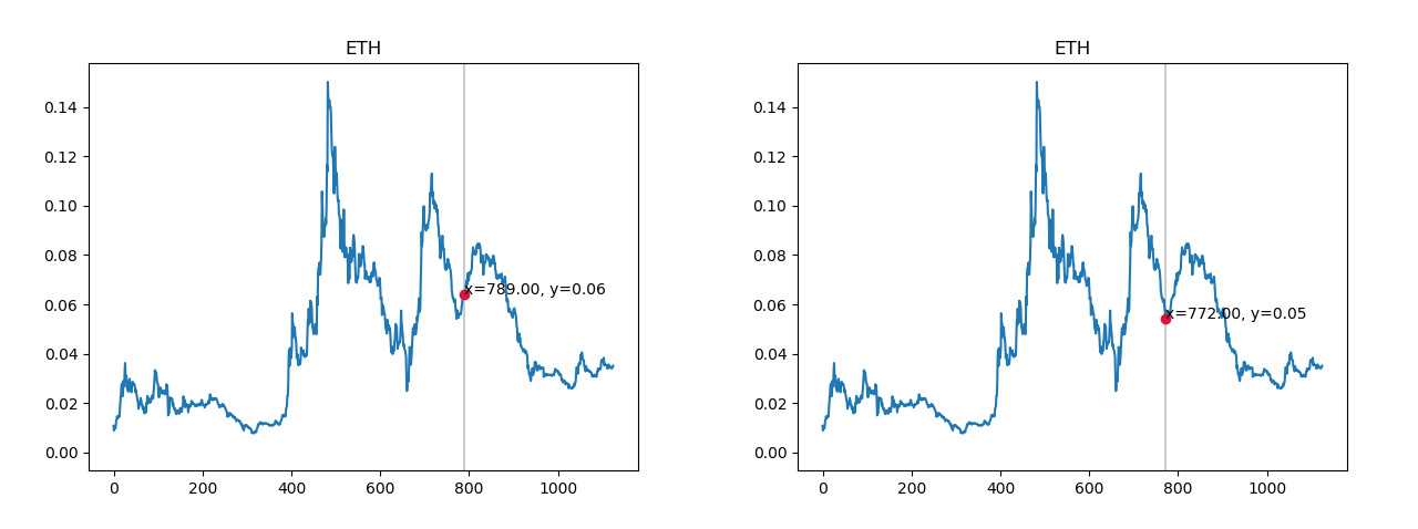
The next step is to graph the price trend and begin spotting areas where we are in a down trend or up trend. These points will be recorded in the coin_up.txt and coin_down.txt files and later be fed into the neural network for training and testing. It is very important to not choose data points that occur before or after a trend because we are not interested in predicting trends, rather we only care about detecting trends.
import pandas as pd
import matplotlib.pyplot as plt
import numpy as np
import os

class SnaptoCursor(object):
    def __init__(self, ax, x, y):
        self.ax = ax
        self.ly = ax.axvline(color="k", alpha=0.2)  # the vert line
        self.marker, = ax.plot([0],[0], marker="o", color="crimson", zorder=3)
        self.x = x
        self.y = y
        self.txt = ax.text(0.7, 0.9, '')

    def mouse_move(self, event):
        if not event.inaxes: return
        x, y = event.xdata, event.ydata
        indx = np.searchsorted(self.x, [x])[0]
        x = self.x[indx]
        y = self.y[indx]
        self.ly.set_xdata(x)
        self.marker.set_data([x],[y])
        self.txt.set_text("x=%1.2f, y=%1.2f" % (x, y))
        self.txt.set_position((x,y))
        self.ax.figure.canvas.draw_idle()

def magnitude_removal(data):
    df = data.copy()
    for i in range(0, len(df)):
        if(df[i] == '-'):
            df[i] = df[i-1]
    mag = df.str.extract(r'[\d\.]+([KMB]+)', expand=False).fillna(1).replace(["K","M","B"], [10**3, 10**6, 10**9]).astype(int)
    base = df.replace(r'[KMB]+$', '', regex=True).astype(float)
    return base*mag

coins = np.array(os.listdir("./coins/"))

for i in range(0, len(coins)):

    dataset = pd.read_csv("./coins/"+coins[i]+"/"+coins[i]+"_raw_daily_data.csv")
    dataset = dataset.dropna()
    dataset = dataset[::-1].reset_index(drop=True)
    close = dataset.loc[:, "Price"]
    close = pd.to_numeric(close, errors="coerce")
    open = dataset.loc[:, "Open"]
    open = pd.to_numeric(open, errors="coerce")
    high = dataset.loc[:, "High"]
    high = pd.to_numeric(high, errors="coerce")
    low = dataset.loc[:, "Low"]
    low = pd.to_numeric(low, errors="coerce")
    vol = dataset.loc[:, "Vol."]
    vol = magnitude_removal(vol)

    t = np.arange(close.size)
    s = close[t]
    fig, ax = plt.subplots()
    cursor = SnaptoCursor(ax, t, s)
    cid =  plt.connect("motion_notify_event", cursor.mouse_move)
    ax.plot(t, s,)
    plt.title(coins[i].upper())
    plt.show()
Below is an example of a good data point vs a bad data point for an upward trend.
Once this data is collected, we can process it with the code shown below. The following code uses the TA-Lib library to calculate the needed technical analysis indicators.
import talib as tl

ema5 = tl.EMA(close, timeperiod=5).rename("EMA5")
ema10 = tl.EMA(close, timeperiod=10).rename("EMA10")
w14 = tl.WILLR(high, low, close, timeperiod=14).rename("W14")
rsi = tl.RSI(close, timeperiod=14).rename("RSI")
mdi = tl.MINUS_DI(high, low, close, timeperiod=14).rename("MDI")
pdi = tl.PLUS_DI(high, low, close, timeperiod=14).rename("PDI")
natr = tl.NATR(high, low, close, timeperiod=14).rename("NATR")
cross = ema5.copy().rename("CROSS")

for j in range(0, ema5.size):
    if(ema5[j] > ema10[j]):
        cross[j] = 1
    else:
        cross[j] = 0

action = close.copy().rename("ACTION")
action = action*0;
print(i)
up = np.loadtxt("./coins/"+coins[i]+"/"+coins[i]+"_up.txt", delimiter='-')
down = np.loadtxt("./coins/"+coins[i]+"/"+coins[i]+"_down.txt", delimiter='-')

for k in range(0, len(up[:])):
    for e in range(int(up[k,0]), int(up[k,1])+1):
        action[e] = 1;
for k in range(0, len(down[:])):
    for e in range(int(down[k,0]), int(down[k,1])+1):
        action[e] = 2;

data = pd.concat([cross, w14, rsi, mdi, pdi, natr, action], axis=1)
data = data.iloc[14:].reset_index(drop=True)
data.to_csv("./coins/"+coins[i]+"/"+coins[i]+".csv")
Pre-Processing the Data
Next, we need to combine all the individual data sets for each coin and split the larger dataset into a training set (70%) and a testing set (30%). Afterwards we apply feature scaling to the input data (technical indicators) and covert the output portion of the data (uptrend/downtrend/no trend) into categorical data.
from sklearn.preprocessing import StandardScaler
sc = StandardScaler()

X = data.iloc[:, 0:len(data.columns)-1].values
y = data.iloc[:,len(data.columns)-1].values
from sklearn.model_selection import train_test_split
X_train, X_test, y_train, y_test = train_test_split(X, y, test_size = 0.3, random_state = 0)
X_train_og = X_train
y_train_og = y_train

# Feature Scaling
from sklearn import preprocessing
scaler = preprocessing.StandardScaler().fit(X_train)
X_train = scaler.fit_transform(X_train)
X_test = scaler.transform(X_test)

# Output to categorical
from keras.utils.np_utils import to_categorical
y_train = to_categorical(y_train)
y_test = to_categorical(y_test)
Training and Testing the Network
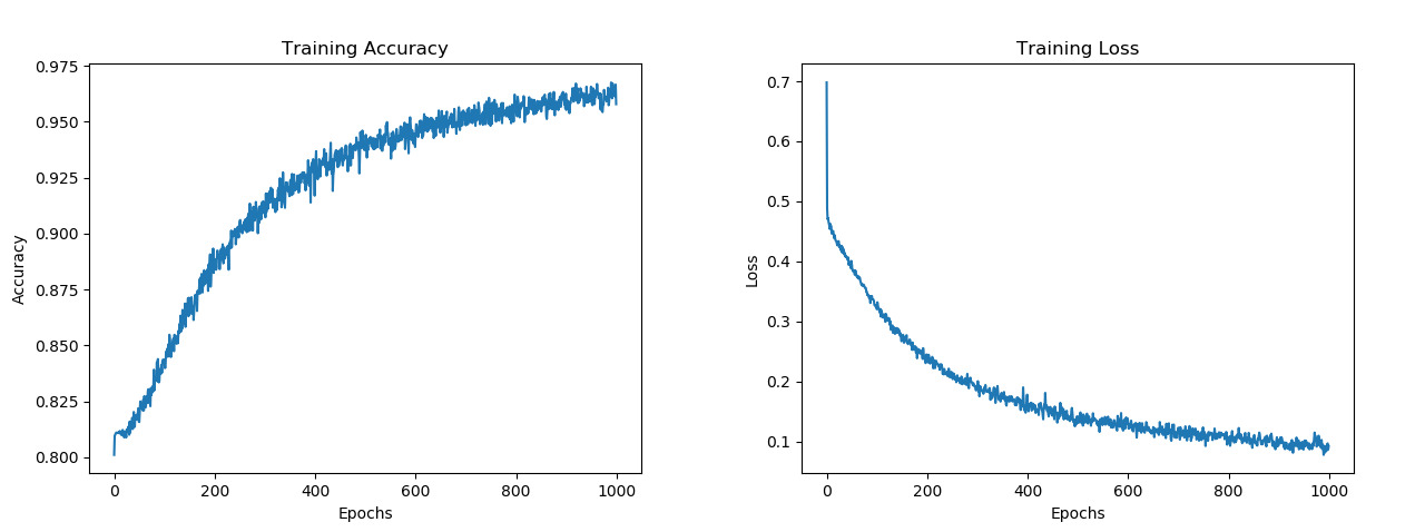
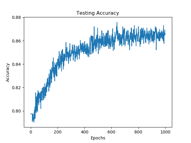
Various network topologies were tested, and the best results were found with networks that have a relatively large number of neurons that progressively get smaller until the output is reached. Adding dropout layers were also largely beneficial in order to create strong meaningful connections. High training accuracies of around 95% were consistently reached and average testing results of 86% were achieved.
from keras.models import Sequential
from keras.layers import Dense
from keras.layers import Dropout

# Building the network
classifier = Sequential()
classifier.add(Dense(units = 1024, kernel_initializer = 'uniform', activation = 'relu'))
classifier.add(Dropout(0.4))
classifier.add(Dense(units = 256, kernel_initializer = 'uniform', activation = 'relu'))
classifier.add(Dropout(0.3))
classifier.add(Dense(units = 64, kernel_initializer = 'uniform', activation = 'relu'))
classifier.add(Dropout(0.2))
classifier.add(Dense(units = 3, kernel_initializer = 'uniform', activation = 'softmax'))
classifier.compile(optimizer = 'adam', loss = 'categorical_crossentropy', metrics = ['accuracy'])

# Fitting the ANN to the Training set
history = classifier.fit(X_train, y_train, validation_data=(X_test, y_test), batch_size = 100, epochs = 1000)

y_pred = np.round(classifier.predict(X_test))
correct_count = 0
for i in range (0,len(y_pred)):
    if( (y_pred[i] == y_test[i]).all()):
        correct_count = correct_count + 1
test_acc = correct_count/len(y_pred)